calcSD
Penis Percentile Calculator
How calcSD makes its calculations
calcSD uses a collection of datasets to make up regional averages. The datasets we use contain researcher-verified measurements with consistent methodology, and we sometimes re-evaluate the datasets currently in use in order to catch potential inaccuracies or biases. With each dataset added/removed, there will be minor changes to the stats. More info about the current datasets is available on the Dataset List page.
We have two different methodologies to determine the statistics, one for most regular measurements, and one for volume.
Length and Girth Stats
For length and girth stats, we use a normal distribution (also known as a Gaussian distribution). This distribution, when plotted into a graph, creates a symmetrical bell curve at the center, with the line going gradually lower and closer to zero as it reaches each end of the graph, creating tails at each end of the distribution. The middle of said distribution can be thought of as the average (or the Mean). Meanwhile, the smoothness of the curve can be thought of as the standard deviation (S.D. or Sigma), where higher values make the probabilities more spread out, and lower values make it more concentrated near the average.
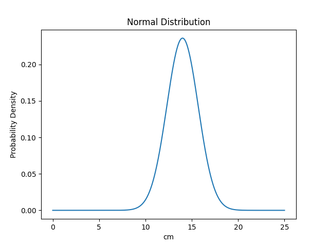
Probability Density Function (μ = 14.00cm, σ = 1.69cm)
At each point of that curve, we can get a value that represents the likelihood (density) that a size falls within that range. The most common value is always the average value, and its exact likelihood depends only on the value of the standard deviation, for example:
| S.D. | Likelihood |
|---|---|
| 0.50 | 0.7979 |
| 0.67 | 0.5954 |
| 1.00 | 0.3989 |
| 2.00 | 0.1995 |
| 3.00 | 0.1330 |
Note that we don't have percentiles quite yet. These values control the height of the curve at its highest point, but they can't be used as probabilities as-is. In order to do that, we have to calculate the integral of that distribution. Yep, that integral, from calculus. Integrals may sound formidable, but the easiest way to make sense of them is that we'll "add up" all of the likelihoods of every point of that graph up until reaching our desired stopping point.
The final formula ends up as follows:
\( F(x) = \int_{-\infty}^{x} \frac{e^{-(x - \mu)^{2}/(2\sigma^{2}) }} {\sigma\sqrt{2\pi}} \)
In the function above, x = input value, e = Euler's number, μ = Mean (average) and σ = Standard deviation.
This formula is what gives us a percentile. At the exact average, the percentile will always be 50%. The rest can be summed up by how far away from the average you are. This is where another concept comes in handy, Z-Scores (sometimes called standard score) which measure how far away you are from the average, it terms of standard deviations. For example, if you are one S.D. away from the average, your Z-Score is ±1, and two away makes a Z-Score of ±2, while being exactly at the average gives a Z-Score of 0. This Z-Score maps nicely to the following percentiles:
| Z-Score | Percentile |
|---|---|
| -3 | 00.13% |
| -2 | 02.28% |
| -1 | 15.87% |
| ±0 | 50.00% |
| +1 | 84.13% |
| +2 | 97.72% |
| +3 | 99.87% |
For some more examples, if the average length is 13cm and the standard deviation is 1cm, then at 14cm your z-score would be +1 which is one SD above the mean. At 16cm you'd have a z-score of +3, at 11cm you'd have a z-score of -2 and so forth.
After a percentile is calculated, it's not difficult to use that rarity to compare against a room of n guys in the end. It's essentially just the percentile subtracted by 100%, then multiplied by the amount of people in the room. And with that, you have the essentials of how calcSD calculates the stats for penis length and girth and other measurements of the like.
Why a normal distribution and not another formula?
The datasets included in calcSD, which are usually scientific studies done by researches, already contain a calculated average and standard deviation, following the expectation of a normal distribution.
Additionally, normal distributions are common in nature and tend to be reliable estimates. While we considered the usage of log-normal distribution, these tend to add an excessive right skew to the average which is inconsistent with the included studies's data at both left and right tails. If penis size is not under appreciable selection, then it is likely to be an accurate approximation.
Unless we end up with enough data to suggest otherwise, a normal distribution will suffice.
Classifications
We also use the percntiles to display size classifications. Where one chooses to place cutoffs for such descriptive classifications is somewhat arbitrary, however for penis size the normal range is medically defined as within 2 SD of the mean, with sizes outside the normal range classified as Abnormally Small or Abnormally Large. Similarly, Micropenis is medically defined as beyond -2.5 SD below the mean, while Macropenis is defined as 2.5 SD above the mean, which each separately correspond to the rarity of ~0.62% of men or an incidence of about 1 in 161 men (technically the definitions of micropenis and macropenis only apply to stretched/erect length, but we may as well apply it to other dimensions too). Additionally, the Statistically Unlikely classification (previously called Theoretically Impossible) is calculated as the size at which the rarity exceeds that of 1 person in the entire global population of males over 15 years of age (~36.8% of 7.7 billion), which corresponds to roughly 6.2 SD from the mean.
Do note that just because a size is determined as impossible in theory, does not mean that it actually is. Biological conditions or just normal genetics can create exceptions in extremely rare cases, much like how the largest human height ever recorded was 8'11", which would be theoretically impossible under the normal approximation to height, since that would be a z-score of well over 12 even when considering just the distribution of heights for men in Western demographics.
This person talks more about how the normal approximation may not be perfect for extreme heights, and hints at a potential issue of our normal distribution's kurtosis and how we might be underestimating the proportions in the extreme tails. The same might also apply to penis size, though with our current data we do not know for sure yet. Regardless, the Statistically Unlikely label offers a rough estimate of the theoretical limit beyond which sizes are not expected to occur in our global population.
Volume Stats
And this is the point where a normal distribution will NOT suffice.
We still need to estimate statistics for the volume of a penis. The volume of the measurements inserted is calculated using the following formula:
\( F(l;c) = l\pi \left(\frac{c}{2\pi}\right)^{2} \)
In the function above, l = length and c = circumference (or girth). Do note we additionaly multiply this result by 0.9 (explained in more detail below).
Assuming a perfectly circular girth shape (not the case in real-life), cross-sectional area of the shaft is calculated, then multiplied by the length of the penis to get a cylindrical approximation of the volume. This cylinder is then corrected by multiplying by 0.9 since penises are typically only occupying close to that proportion of a perfect cylinder (obviously this approximation doesn't accurately predict the volume of every penis since some are very non-uniform, however it should on average improve the estimate by correcting for volume reductions from the indentation below the coronal ridge, the conical head, and the imperfectly circular circumference).
The distribution for volume however, is way more complicated. To calculate that, we'd need either paired data of lengths and girths. Unfortunately paired data is not readily available, so the most reliable method of determining volume is already out of the question. We do have studies that have contributed their correlation values between length and girth though, which is still useful.
The correlation coefficients we have grabbed are as follows:
BPEL - Erect Girth: r = 0.55
NBPEL - Erect Girth: r = 0.40
An alternative is to mix two normal distributions together using a correlation value, thus gaining a multivariate normal distribution. This allows us to create our own pairs of length and girth data based on the existing statistics. Unfortunately, this is still not enough to estimate volume as the volume of 200ml may be achieved with a size of 16.5cm of length by 13cm of girth (which falls slightly outside average range and thus should be commonly expected) but also by a size of 13cm by 14.5cm, which is significantly more uncommon. Calculating the rarity of a specific size then would exclude the rarity of other sizes which may have the same volume.
Up until v3.4 of calcSD we used a different method (see section below) but we switched away due having some technical difficulties with it.
Volume stats follow the log-normal and power-normal distribution functions fairly well, with log-normal being more accurate below the average, and power-normal being more accurate above. Neither are a 1-to-1 match with our former method, but we decided to go with power-normal distribution due to it being the most accurate one overall.
A power normal distribution is a distribution of a random variable where its exponentiation is normally distributed. For our purposes, this means that, if penis volume is x, then x is not normally distributed, but xy is. The exact details are more complicated, and it involves redefining some concepts we used previously.
For starters, in order to find the percentile for a power normal distribution, the function is as follows:
\( F(x;\lambda) = 1 - (\Phi(-(\frac{x-\mu}{\sigma})))^{\lambda} \)
In the function above, x = input value, μ = Location, σ = Scale and λ = Shape. Additionally, x and λ must be higher than 0.*
There's also another symbol: Φ represents the normal distribution formula from earlier. Everything that's inside Φ(...) in the power normal distribution will be inputted into the F(x) of the normal distribution. There's one catch: in this case, when solving the normal distribution, we'll always use μ=0 and σ=1. This is called the standard normal distribution.
This also means that unlike before, these variables don't correspond directly to the mean and average of the distribution. calcSD calculates these values (alongside the rest of the variables above) using SciPy by feeding it the sampled data from the multivariate distribution from earlier, and then fitting it to the most appropriate values for the power normal distribution.
While SciPy is needed for this step, once we have these parameters calculated, we can use the formula directly in the browser to achieve a percentile given a location, scale and shape parameter. This is how calcSD calculates volume stats. While we still display an average (mean), the meaning of "standard deviation" and "Z-Score" become lost and as such we don't put as much emphasis on these numbers.
Besides, if the regular stats are just an estimate, volume stats are even more of an estimate, and even further removed from the original data.
* Having these be larger than 0 is not a problem for us given penis volume is always positive.
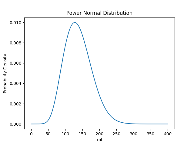
Probability Density Function (μ = 79.36868, σ = 15.64903, λ = 0.08167)
calcSD v3.4 and older
Previously, in order to calculate the volume rarity we used the volumes of each of the length and girth pairs generated in the multivariate normal distribution, and then created a gaussian mixture model of the generated volume data. The resulting distribution was very close to a normal distribution, however, it had a right skew which caused a large differences in the tails (for constant length and a normal approximation to the volume, to get the same percentile as the multivariate distribution in some cases it can correspond to more than half an inch less girth). This difference is because the distribution of volume is not normal, which is known from the math behind the product of normal variables.
These calculations were fairly intensive, and could not be done on the fly. We used to have a file containing precalculated volumes for every 0.5ml increment and their relevant percentiles. A separate file for each dataset, for NBPEL and BPEL. Yeah.
Doing things this way introduced a lot of problems, mainly caused by the inaccurate integration being done (of which we couldn't easily optimize due to lack of familiarity with Python, the stats involved and due to existing integration functions taking forever with our custom code), and it was also a waste of bandwidth.
Some datasets with high standard deviation broke easily with stats near the "Statistically Unlikely" area of ±6.2 SD, requiring increasing amounts of spaghetti to fix, and at one point it was just too tricky to leave as it was, as such, it was retired for a less accurate but more "well-behaved" method, from a programming standpoint, as outlined earlier.
Regional Averages
Regional averages are actually a type of dataset that calcSD internally calls "aggregates". To join multiple different datasets together, the sample size of each measurement type (length, girth, etc.) is added up. The average and standard deviation of said measurement type in each dataset is then divided by the total amount of samples in all datasets and multiplied by the total amount of samples in that specific dataset. An easy example is detailed over on the old version of calcSD. Note that the calcSD Averages described there are outdated and no longer used.
We are looking into changing how this data is added up to see if we can improve its accuracy by using a methodology similar to how volume is calculated above: by simulating samples from each dataset, then estimating an average based on the samples created. This or a different methodology, or perhaps multiple different ones, might be used in a future update.
Quirks and Trivia
- Want to know how to pronounce those greek letters? μ = mu, σ = sigma, λ = lambda and Φ = phi. Also, π = pi but you likely already knew that one.
- The functions displayed above, for calculating the percentiles, are more formally known as "Cumulative Distribution Functions" or CDFs.
- Power normal distributions cause the -6.2 SD "Statistically Unlikely" classification to glitch out and predict negative volumes. We are temporarily fixing it by quietly changing it to -5.2 SD instead, but in the future we'll take a look at our calculations more closely to see where this discrepancy is coming from. This does not affect our normal distribution stats (length/girth).
- The 0 and 100 percentiles don't exist. Saying you're in the 99 percentile means you're higher than 99% of the population, but saying you're on the 100 percentile means you're higher than 100% of the population, including yourself... which is a contradiction! Same goes for the 0 percentile but in reverse.
- calcSD displays rounded numbers to you, but the calculations themselves are used with as many decimal places as allowed by our code, meaning if you try to do the math yourself using the rounded average and standard deviation (S.D.) we display, you might get a less accurate percentile result than what we display.
- While SciPy has been of much help for these stats, we also would like to thank some sources from the NIST, specifically these pages for normal distribution and power normal distribution.
- For the in-browser stats, we use GoNum alongside some of our own custom code, compiled to WebAssembly, to speed things up and provide more accurate results.